영상에서 추출한 프레임들의 종횡비를 고려하지 않은 채 224 x 224 로 리사이즈하여 생겼던 왜곡을 다시 원상태로 돌리고, 모델을 다시 돌려봐야하는 단계에서 Bi-LSTM + Attention 모델로 변경하는 것이 어떨지에 대한 얘기가 회의 중에 나와서 관련 논문을 읽고 비교를 해본다.

관련 논문과 정리 내용

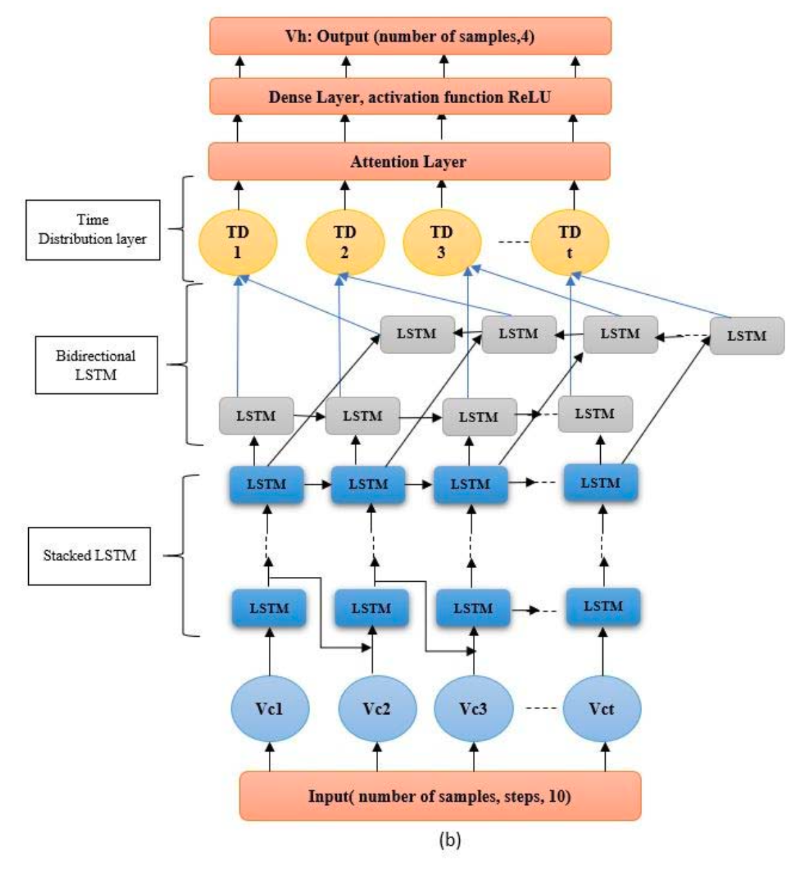
Detecting Driver Behavior Using Stacked LSTM Network With Attention Layer

목적, 마감, 결과, subtasks

Bi-LSTM 원리

💡

핵심 아이디어

Bi-LSTM은 입력 시퀀스를 두 방향(정방향, 역방향)으로 동시에 처리함으로써, 각 시점의 출력을 계산할 때 이전 정보(과거) 뿐만 아니라 이후 정보(미래)도 함께 고려함

구조

X = [x₁, x₂, x₃, x₄, x₅]

Bi-LSTM은 두 개의 LSTM을 사용

Forward LSTM (→)

입력 시퀀스를 정방향으로 처리

x₁ → x₂ → x₃ → x₄ → x₅

각 시점의 출력(hidden state)

h₁^→ = LSTM_forward(x₁)
h₂^→ = LSTM_forward(x₂)
h₃^→ = LSTM_forward(x₃)
h₄^→ = LSTM_forward(x₄)
h₅^→ = LSTM_forward(x₅)

Backward LSTM (←)

입력 시퀀스를 역방향으로 처리

x₅ → x₄ → x₃ → x₂ → x₁

입력은 뒤에서부터 처리되지만, 출력은 시간 순서대로 매핑

h₁^← = LSTM_backward(x₁)
h₂^← = LSTM_backward(x₂)
h₃^← = LSTM_backward(x₃)
h₄^← = LSTM_backward(x₄)
h₅^← = LSTM_backward(x₅)

시간 t에서의 bi-LSTM의 은닉 상태는 다음처럼 구성됨

h_t = [h_t || h_t]

|| 는 벡터 결합(concatenation) 연산

항목	단일 LSTM	Bi-LSTM
입력 시퀀스	T	T
출력 벡터 차원	hidden_size	2 x hidden_size
출력 텐서 shape	(T, hidden_size)	(T, 2 x hidden_size)

forward, backward 결과를 벡터 결합하기 때문에 출력의 수(T)는 동일하지만, 동일한 LSTM 성능을 유지하고 싶다면 hidden_size는 두 배 해야함

시각적 다이어그램

Input Sequence:  x₁       x₂       x₃      ...     x₁₂

Forward LSTM:    h₁^→ →  h₂^→ →  h₃^→  ...    h₁₂^→
Backward LSTM:   h₁^← ←  h₂^← ←  h₃^←  ...    h₁₂^←

Final Output:    h₁ = [h₁^→ ; h₁^←]
                 h₂ = [h₂^→ ; h₂^←]
                 ...
                 h₁₂ = [h₁₂^→ ; h₁₂^←]

Bi-LSTM + Attention 도입 시 기대되는 장점

높은 예측 정확도	Bi-LSTM은 과거 + 미래 맥락을 모두 활용하고 Attention은 유용한 정보에 집중함으로써, 두 기법의 상호 보완적 효과로 모델 정확도가 향상 논문에서 제안된 모델은 기존 단뱡항 LSTM 대비 오류율을 크게 감소시켰으며, 이는 미래 정보를 반영한 은닉표현과 중요 입력의 강조 덕분
일반화 성능 향상 및 오버피팅 완화	Attention 메커니즘은 불필요한 정보에 대한 가중치를 낮추고 핵심적인 입력에만 높은 가중치를 할당하기 때문에, 모델이 훈련 데이터의 잡음까지 암기하는 것을 막아줌 그 결과, 논문에서도 학습 오차와 테스트 오차의 차이가 크게 줄어들어(오버피팅 감소) 모델의 일반화 성능이 개선됨
학습 속도 향상 및 효율성	Attention을 통해 모델이 중요한 부분에 집중하여 학습함으로써 훈련 과정이 빨라지고 수렴이 빠르게 이루어지는 장점이 있음 논문에서도, attention을 추가한 모델은 더 적은 에폭으로 동일 성능에 도달하여 연산 비용을 절감했다고 보고함 Attention 레이어가 메모리 역할을 수행하여 LSTM이 모든 정볼르 일렬로 압축해야하느 부담을 줄여주기 때문
모델 해석력 향상	Attention 가중치는 각 입력 시퀀스 요소의 중요도를 나타내므로, 어떤 요인이 운전자 행동에 영향을 주었는지를 해석할 수 있는 단서를 제공

LSTM 셀 구조

               ┌────────────┐
      x_t ────▶│            │
     h_{t-1}──▶│   LSTM     │──▶ h_t   (출력)
     c_{t-1}──▶│   Cell     │──▶ c_t   (업데이트된 셀 상태)
               └────────────┘

LSTM의 셀 개수는 시퀀스 길이와 같음

LSTM 셀 = LSTM이 하나의 시점 t를 처리하는 작은 모듈

→ bi-LSTM은 시퀀스 길이 T만큼의 forward 셀, backward 셀 각각 있으므로 시퀀스 길이의 2배만큼 셀이 있음

hidden state 크기

각 시점 t에서 LSTM이 출력하는 은닉 상태 $h_i$ 의 벡터 차원

예를 들어, hidden size=64이면, $h_t \in \mathbb{R}^{64}$ 이고, 전체 시퀀스 출력은 shape이 (T, 64)가 됨 (T: 시퀀스 길이)

hidden state 는 각 시점에서 LSTM이 얼마나 풍부하게 정보를 표현하느냐 결정

즉, 하나의 셀이 얼마나 복잡한 특징을 기억할 수 있는지, 메모리 용량 같은 개념

결정하는 법

경험 기반
모델 규모 추천 hidden size
작거나 빠르게 학습하고 싶을 때 16, 32
보통 수준의 데이터 64, 128
복잡한 문제, 더 깊은 특징 표현 필요 256, 512 이상

문제의 복잡도 기준
- 예측해야 하는 출력이 단순하거나 데이터 양이 적다면 → 작은 크기
- 시계열 길이가 길고, 복잡한 패턴이 많다면 → 큰 크기

오버피팅 여부 확인
- hidden size가 너무 크면
  - 훈련 데이터에 지나치게 적합(overfit)
  - 학습 시간이 길어지고 성능이 불안정
- 너무 작으면
  - 충분한 표현을 못 해서 underfit
검증 성능 기준으로 Grid Search 나 Validation loss를 통해 최적화

Time Distribution layer

	TimeDistributed(Dense)	Dense
차이점	시퀀스의 각 시점마다 동일한 Dense를 반복 적용	전체 시퀀스를 1개의 벡터처럼 보고 Dense 한 번만 적용
시계열 시점 유지	O	X
입력 shape	(batch, time, features)	(batch, features) or flatten
출력 shape	(batch, time, new_features)	(batch, new_features)

꼭 attention 전에 hidden size를 줄여야할까?

상황	추천 전략
LSTM hidden size가 크고 연산이 부담됨	TimeDistributed(Dense(small_dim))로 줄이고 Attention
Attention layer가 dot-product 방식일 때	줄이는 게 매우 유리 self-attention에서 사용되는 대표적인 방식
성능이 중요하고 연산량 문제 없음	hidden size 그대로 유지
실험 중이라면?	둘 다 해보고 validation loss로 비교해보기

논문 구조 코드화

TensorFlow / Keras 버전

from tensorflow.keras.layers import Input, LSTM, Bidirectional, TimeDistributed, Dense, Attention, Layer
from tensorflow.keras.models import Model
import tensorflow as tf

class AdditiveAttentionLayer(Layer):
    def __init__(self, units):
        super(AdditiveAttentionLayer, self).__init__()
        self.W1 = Dense(units)
        self.W2 = Dense(units)
        self.V = Dense(1)

    def call(self, encoder_output):
        # encoder_output: (batch_size, time_steps, hidden_size)
        score = self.V(tf.nn.tanh(self.W1(encoder_output)))
        attention_weights = tf.nn.softmax(score, axis=1)
        context_vector = attention_weights * encoder_output
        context_vector = tf.reduce_sum(context_vector, axis=1)  # (batch_size, hidden_size)
        return context_vector

# 모델 구성
input_ = Input(shape=(12, 10)) # time_steps, feature_dim

# Stacked LSTM + BiLSTM
x = LSTM(64, return_sequences=True)(input_)
x = LSTM(64, return_sequences=True)(x)
x = Bidirectional(LSTM(64, return_sequences=True))(x)

# TimeDistributed(Dense)
x = TimeDistributed(Dense(64, activation='relu'))(x)

# Additive Attention
context = AdditiveAttentionLayer(units=64)(x)

# Output
output = Dense(4, activation='linear')(context)

model = Model(inputs=input_, outputs=output)
model.summary()

python

Pytorch

import torch
import torch.nn as nn
import torch.nn.functional as F

class AdditiveAttention(nn.Module):
    def __init__(self, hidden_dim, attn_dim):
        super(AdditiveAttention, self).__init__()
        self.W1 = nn.Linear(hidden_dim, attn_dim)
        self.V = nn.Linear(attn_dim, 1)

    def forward(self, encoder_output):
        # encoder_output: (batch, time_steps, hidden_dim)
        score = self.V(torch.tanh(self.W1(encoder_output)))  # (batch, time_steps, 1)
        weights = torch.softmax(score, dim=1)                # (batch, time_steps, 1)
        context = torch.sum(weights * encoder_output, dim=1) # (batch, hidden_dim)
        return context, weights

class BiLSTM_Attention_Model(nn.Module):
    def __init__(self, input_dim=10, lstm_dim=64, attn_dim=64, output_dim=4):
        super(BiLSTM_Attention_Model, self).__init__()
        # num_layers = 2와 같음
        self.lstm1 = nn.LSTM(input_dim, lstm_dim, batch_first=True, bidirectional=False)
        self.lstm2 = nn.LSTM(lstm_dim, lstm_dim, batch_first=True, bidirectional=False)
        self.bi_lstm = nn.LSTM(lstm_dim, lstm_dim, batch_first=True, bidirectional=True)
        self.fc_time = nn.Linear(lstm_dim * 2, lstm_dim)
        self.attn = AdditiveAttention(lstm_dim, attn_dim)
        self.output_layer = nn.Linear(lstm_dim, output_dim)

    def forward(self, x):
        x, _ = self.lstm1(x)         # (batch, seq, lstm_dim)
        x, _ = self.lstm2(x)         # (batch, seq, lstm_dim)
        x, _ = self.bi_lstm(x)       # (batch, seq, lstm_dim*2)
        x = F.relu(self.fc_time(x))  # TimeDistributed(Dense) equivalent
        context, weights = self.attn(x)  # (batch, lstm_dim), (batch, time_steps, 1)
        output = self.output_layer(context)  # (batch, output_dim)
        return output, weights

python

Bi-LSTM + Attention 모델로 변경 고민

Bi-LSTM 원리

구조

시각적 다이어그램

Bi-LSTM + Attention 도입 시 기대되는 장점

LSTM 셀 구조

hidden state 크기

결정하는 법

Time Distribution layer

꼭 attention 전에 hidden size를 줄여야할까?

논문 구조 코드화

TensorFlow / Keras 버전

Pytorch

Tags

모델 규모	추천 hidden size
작거나 빠르게 학습하고 싶을 때	16, 32
보통 수준의 데이터	64, 128
복잡한 문제, 더 깊은 특징 표현 필요	256, 512 이상

sol’s blog

Bi-LSTM + Attention 모델로 변경 고민

Bi-LSTM 원리

구조

시각적 다이어그램

Bi-LSTM + Attention 도입 시 기대되는 장점

LSTM 셀 구조

hidden state 크기

결정하는 법

Time Distribution layer

꼭 attention 전에 hidden size를 줄여야할까?

논문 구조 코드화

TensorFlow / Keras 버전

Pytorch

Tags